Lesson 5 · How a Model Learns

In Lesson 4 you built one transformer block and stacked it. Put a token embedding in front and an output head behind, and that stack becomes a complete language model. Let's assemble a real one — the GPT-2 architecture — from OLM parts, and then teach it to write.

Keep your Colab notebook open.

A whole GPT-2, from scratch

GPT-2 is nothing more than the pieces you already know, arranged in a set order: a token embedding, a positional embedding (so the model knows word order), a stack of transformer blocks, and an output head. Here's the architecture next to the OLM code that builds each part:

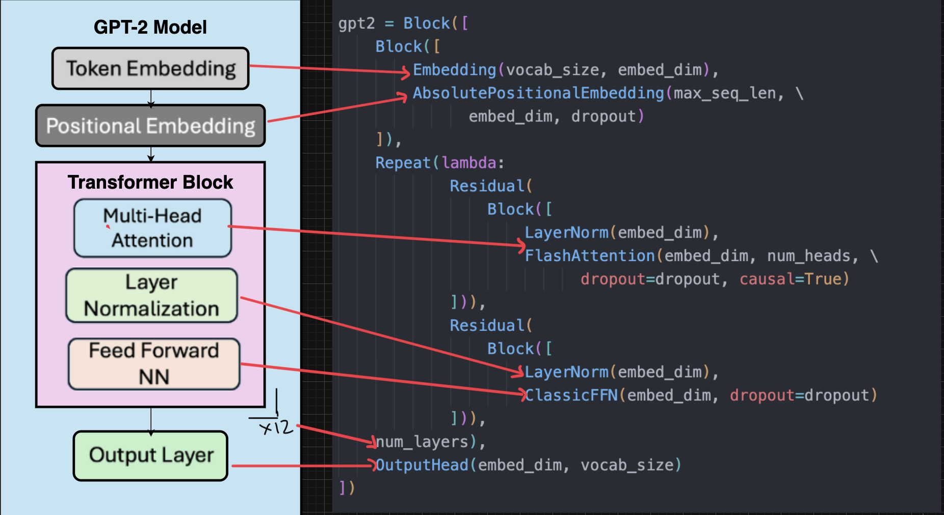
The output head is the final prediction layer. It turns each final vector into a score for every token in the vocabulary, and softmax turns those scores into next-word probabilities.

And here it is in code — read it against the picture, piece by piece:

from olm.data.tokenization import HFTokenizer
from olm.nn.structure import Block
from olm.nn.structure.combinators import Residual, Repeat
from olm.nn.embeddings import Embedding, AbsolutePositionalEmbedding
from olm.nn.attention import MultiHeadAttention
from olm.nn.feedforward import ClassicFFN
from olm.nn.norms import LayerNorm
from olm.nn.blocks import OutputHead

tok = HFTokenizer("gpt2")

embed_dim   = 768     # numbers per token
num_heads   = 12      # attention heads in each block
num_layers  = 12      # transformer blocks in the stack
max_seq_len = 1024    # longest sequence it can read

gpt2 = Block([
    Embedding(tok.vocab_size, embed_dim),                 # tokens → vectors        (Lesson 2)
    AbsolutePositionalEmbedding(max_seq_len, embed_dim),  # add word-order info
    Repeat(lambda: Block([                                # the stack of blocks     (Lesson 4)
        Residual(Block([LayerNorm(embed_dim), MultiHeadAttention(embed_dim, num_heads, causal=True)])),
        Residual(Block([LayerNorm(embed_dim), ClassicFFN(embed_dim)])),
    ]), num_layers),
    OutputHead(embed_dim, tok.vocab_size),                # vectors → a score per token
])

n_params = sum(p.numel() for p in gpt2.parameters())
print(f"{n_params/1e6:.0f}M parameters")

That's it — that's GPT-2, built from the same handful of parts you met over the last three lessons. The print shows it holds well over a hundred million numbers.

Right now, it knows nothing

Every one of those hundred-million-plus numbers — the model's weights — started at a random value. Feed "The cat sat on the" into this fresh model and its guess for the next token is essentially a coin toss across the whole vocabulary. Training is how those random numbers turn into ones that predict real language — through practice.

The loop: guess, score, nudge, repeat

Training is a loop. One round of it goes like this:

1. Guess. Take a chunk of real text and feed it in. At every position, the model predicts the next token.
2. Score. Compare each prediction to the token that actually came next, and boil the result down to a single number — the loss — that says how wrong the model was. A big loss means very wrong.
3. Nudge. Adjust every weight a tiny amount, in the direction that would have made the loss a little smaller.
4. Repeat. Do it again with the next chunk of text. Millions of times, over mountains of text.

Slowly, the random numbers settle into values that predict real language well. That's all training is — the same four steps, over and over.

The clever part is step 3. You never work out those adjustments yourself: an algorithm called backpropagation figures out, for every weight, which way to nudge it, and an optimizer applies the nudges. You can train models your whole life without ever doing that calculation by hand.

Reading the numbers while it trains

As a model trains, you mostly watch two numbers:

• Loss — the "how wrong" number from step 2. It starts high and should drift down as training goes on. A falling loss is the sign it's working.
• Perplexity — a friendlier way to read the loss: roughly, "how many tokens was the model torn between?" A perplexity of 20 means it was about as unsure as picking among 20 equally likely words. Perplexity of 1 would be perfect. Lower is better.

Two more words you'll see:

• Learning rate — how big each nudge is. Too big and training is unstable; too small and it crawls.
• Epoch / step — an epoch is one full pass over your data; a step is one nudge (one round of the loop).

What the loop looks like in code

Because OLM models are ordinary PyTorch, the heart of training is only a handful of lines. You won't run this snippet — it's here just to show how little there is to it:

for inputs, targets in data:              # a chunk of text, and what comes next
    predictions = model(inputs)           # 1. guess
    loss = loss_fn(predictions, targets)  # 2. score
    loss.backward()                       # 3. work out the nudges
    optimizer.step()                      #    apply them
    optimizer.zero_grad()                 #    reset for the next round

That's the whole idea: guess, score, nudge, reset, repeat.

Letting OLM run the loop

In practice you don't write that loop by hand — OLM's Trainer runs it for you and handles the practical details (batching, the learning-rate schedule, reporting). You hand it a model, an optimizer, and your data, and call train:

from olm.train import Trainer

trainer = Trainer(model, optimizer, loader, device, context_length=128)
losses = trainer.train(epochs=1, max_steps=100)

Each step, it does exactly the four things above and prints the loss falling as the model learns.

You've finished the foundations

Stop and look at what you can now explain: text becomes tokens and then embeddings; attention lets words share context; blocks stack into a transformer; an embedding and output layer make it a full model; and training nudges its random weights into one that predicts real language. That's the whole shape of how a language model works.

Now it's time for the payoff: do it for real, end to end, on actual text. The next tutorial uses a much smaller GPT-style model so you can train it, watch the loss fall, and generate text in the same session:

Next: Your First Language Model

Want to know exactly how attention computes which words matter — queries, keys, and all? That's the one piece we treated as a black box. It's written up in How Attention Works (deep dive) — entirely optional, and a good read once the rest has settled.